Dynamic Programming Patterns: The Ultimate Guide

Dynamic Programming (DP) is a powerful technique to solve problems by breaking them into overlapping subproblems and reusing solutions. It often feels tricky at first, but most DP challenges fall into a few common patterns. Recognizing these patterns is key to mastering DP for competitive programming and top tech interviews. In this guide, we’ll explore major DP patterns – including 0/1 Knapsack, Unbounded Knapsack, Subset Sum, Longest Common Subsequence, Longest Increasing Subsequence, DP on Trees, DP on Grids, and Palindrome problems – and provide detailed explanations, decision logic, tips, and JavaScript code examples (top-down vs bottom-up) for each. We’ll also discuss space optimizations and list practice problems (primarily from LeetCode) to solidify each pattern.

Whether you’re optimizing item selection under constraints, finding subsequences, or counting paths in a grid, understanding the underlying pattern will help you map a new problem to a known DP solution. Let’s dive in!

0/1 Knapsack Pattern

The 0/1 Knapsack pattern is a classic DP scenario where you decide to take an item or leave it. It arises in problems where you have a set of items, each with a value and a weight (or cost), and you want to maximize the total value without exceeding a weight capacity (Knapsack problem - Wikipedia). The term "0/1" indicates that each item can be chosen at most once – you either take an item (1) or you don’t (0). This pattern appears in resource allocation problems where you must choose an optimal subset under constraints (e.g. selecting projects under a budget). A real-world analogy is a thief trying to fill a knapsack with the most valuable combination of goods without exceeding the bag’s weight limit (Knapsack problem - Wikipedia).

• Common Problem Structures: Selecting a subset of elements to maximize sum value under a weight/volume constraint, or to achieve an exact sum. Examples include the classic Knapsack Problem, Subset Sum, Partition Equal Subset Sum, Target Sum, and choosing non-adjacent items for max sum (related to House Robber problem).

• Key Idea: For each item, you have two choices – include it or exclude it – and you use previous results to decide. This yields a recurrence of the form: dp[i][w] = max(dp[i-1][w], value[i] + dp[i-1][w - weight[i]]). In other words, at item i and capacity w, you compare not taking the item (value stays as for previous item at same capacity) vs. taking it (add item’s value and use remaining capacity’s best from previous items).

• Decision-Making Logic: Build solutions for smaller subproblems (fewer items or smaller capacity) and use them to solve larger ones. The DP state typically is dp[i][w] = best value using first i items within capacity w. Base cases: dp[0][*] = 0 (no items yields 0 value) and dp[*][0] = 0 (zero capacity yields 0 value). Each new item introduces a binary choice (take or skip), leading to the optimal substructure.

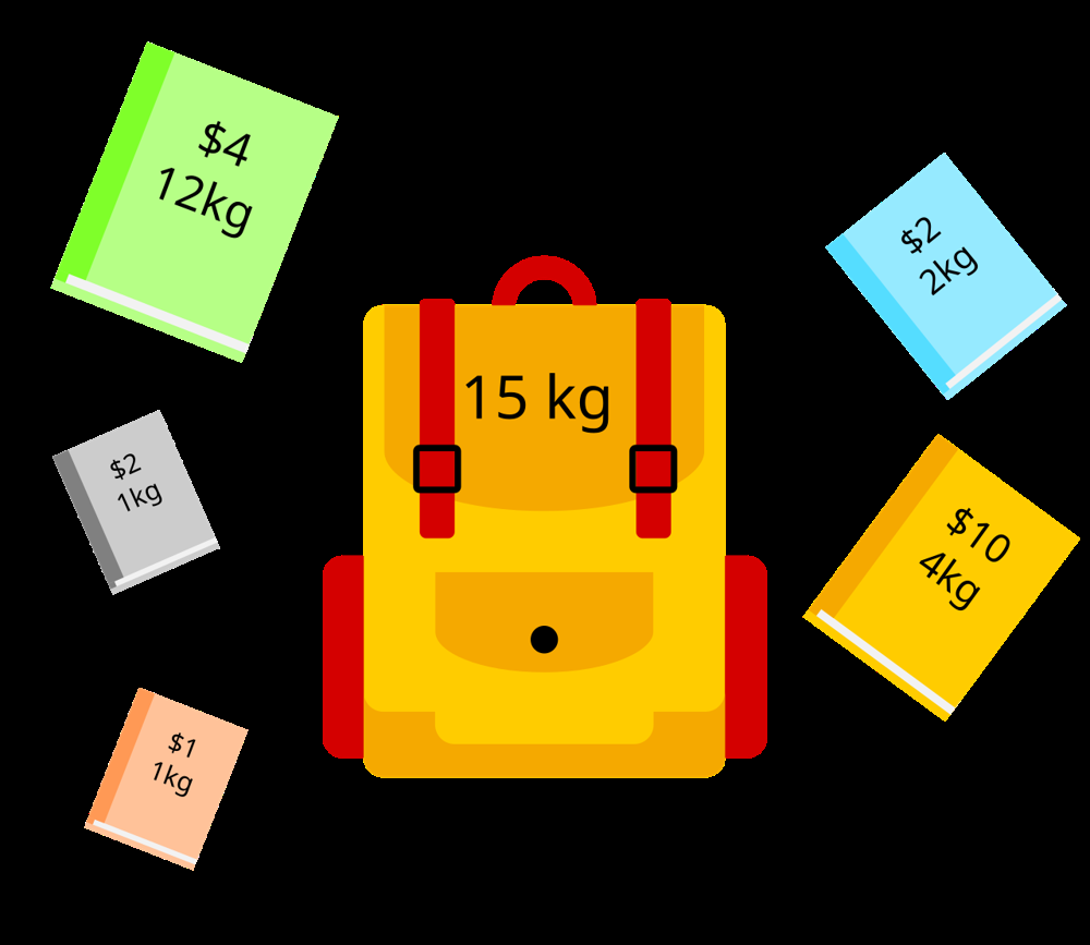
Figure: 0/1 Knapsack illustration – choosing items (books with weights and values) to maximize value within a 15kg capacity. Each book can be taken (1) or not taken (0), and the optimal combination here fills the knapsack to exactly 15kg without exceeding it.

Top-Down vs Bottom-Up Approaches

Top-Down (Memoization): We formulate a recursive solution and memoize overlapping subproblems. For knapsack, define a recursive function knap(i, remainingWeight) that returns the best value using items 0..i with remaining capacity. The recursion explores both choices (include item i if it fits, or exclude it), and stores results in a memo table (e.g. a 2D array or dictionary keyed by (i, remainingWeight)). This approach is intuitive – it mirrors the problem’s decision tree (include/exclude at each step) and uses caching to avoid recomputation (Dynamic Programming-Parent Problem 1 (0/1 Knapsack): 3 approaches with practice questions. | by Eva Sharma | Medium) (Dynamic Programming-Parent Problem 1 (0/1 Knapsack): 3 approaches with practice questions. | by Eva Sharma | Medium). The memoization table size is n * W (number of items × capacity). Time complexity is reduced from exponential to O(n * W) by caching results.

Bottom-Up (Tabulation): We iteratively build a DP table for subproblem sizes from small to large. For knapsack, we create a table dp[n+1][W+1] where dp[i][w] represents the best value using first i items and capacity w. We start with base cases (dp[0][w] = 0 for all w, dp[i][0] = 0 for all i) and fill the table row by row. When filling dp[i][w], we use the recurrence described above. This approach ensures we solve all subproblems in a controlled manner and is often slightly more space-efficient in terms of call stack (no recursion). It also makes it straightforward to apply space optimizations.

Below are JavaScript examples for 0/1 Knapsack using both approaches. Suppose we have weights, values arrays and a knapsack capacity. (This could model, for example, selecting projects with certain costs and profits under a budget limit.)

Top-Down (Memoization) Example – 0/1 Knapsack

// Top-Down 0/1 Knapsack in JavaScript
function knapSackTD(weights, values, capacity) {
  const n = weights.length;
  // Memo table for states (i, cap) initialized to undefined
  const memo = Array.from({ length: n }, () => ({}));

  function dfs(i, cap) {
    // Base case: no items or no capacity
    if (i < 0 || cap === 0) return 0;
    if (memo[i][cap] !== undefined) {
      return memo[i][cap]; // Return cached result if available
    }
    // Option 1: exclude this item
    let best = dfs(i - 1, cap);
    // Option 2: include this item (if it fits)
    if (weights[i] <= cap) {
      best = Math.max(best, values[i] + dfs(i - 1, cap - weights[i]));
    }
    memo[i][cap] = best; // Memoize result
    return best;
  }

  return dfs(n - 1, capacity);
}

Explanation: We use dfs(i, cap) to compute the best value using items up to index i for a given remaining capacity cap. We try excluding the item i and including it (if possible), and take the max. The memoization (using a JS object for each i or could use a 2D array) ensures each subproblem is solved once.

Bottom-Up (Tabulation) Example – 0/1 Knapsack

// Bottom-Up 0/1 Knapsack in JavaScript
function knapSackBU(weights, values, capacity) {
  const n = weights.length;
  // dp[i][w] = max value using first i items (1-indexed for convenience) and capacity w
  const dp = Array.from({ length: n + 1 }, () => Array(capacity + 1).fill(0));

  for (let i = 1; i <= n; i++) {
    for (let w = 0; w <= capacity; w++) {
      if (weights[i-1] <= w) {
        // Max of including item (i-1) or not
        dp[i][w] = Math.max(values[i-1] + dp[i-1][w - weights[i-1]], dp[i-1][w]);
      } else {
        // Cannot include item (i-1)
        dp[i][w] = dp[i-1][w];
      }
    }
  }
  return dp[n][capacity]; // result for all items and full capacity
}

Explanation: We build the table row by row. dp[i][w] references dp[i-1][*] (previous row), which ensures we only use each item once (since when considering item i, we only look at solutions without it from the previous row). The answer ends up in dp[n][capacity]. This approach also runs in O(n * capacity) time.

Space Optimization and Tips

A neat optimization for 0/1 knapsack is reducing space from O(n*W) to O(W). Notice that to compute row i, we only need row i-1. We can use a 1D array dp[w] and update it in reverse weight order (from W down to 0) when processing each item (0/1 Knapsack Problem - Dynamic Programming - Taro). Reversing the loop ensures that when we update dp[w] for including the current item, we still have the results from the previous item (since smaller weights have not yet been updated in this iteration). For example:

// Space-optimized 0/1 Knapsack
function knapSackOptimized(weights, values, capacity) {
  const dp = Array(capacity + 1).fill(0);
  for (let i = 0; i < weights.length; i++) {
    for (let w = capacity; w >= weights[i]; w--) {
      dp[w] = Math.max(dp[w], values[i] + dp[w - weights[i]]);
    }
  }
  return dp[capacity];
}

This yields the same result with O(W) space. Use this trick for large constraints where memory is an issue.

Tips & Tricks:

• If asked for just a yes/no or count of ways to meet a sum (as in Subset Sum or variation), you can often use a boolean or count DP array similarly. The 0/1 Knapsack logic can be adapted to check if a sum is achievable (using booleans) or count the number of ways (using addition instead of max).

• Look for phrases like “choose a subset”, “within a budget/limit”, “maximize value/profit” – these hint at knapsack patterns. Also, if each element can only be picked once, it’s 0/1 knapsack.

• Ensure you handle edge cases: zero capacity or no items usually yields 0, and you may need to handle cases where no valid selection is possible (sometimes by initializing DP with -Infinity for impossible states).

Related Problems: Partition Equal Subset Sum, Target Sum, and others (see problem list at end) are direct applications of this pattern. Mastering knapsack helps in many variations of subset selection and optimization problems.

Unbounded Knapsack Pattern

The Unbounded Knapsack pattern is a variation where you can use items an unlimited number of times. This appears in coin change problems, integer partitioning, and any scenario where the supply of each item is infinite. The problem setup is similar to 0/1 knapsack (items with weight/cost and value), but unlike 0/1, you can pick an item multiple times. A classic real-world example is making change for an amount using given coin denominations – you can use each coin type as many times as needed.

• Common Problem Structures: Coin Change (minimum coins to make a sum), Coin Change 2 (count ways to make a sum), Rod Cutting (max profit by cutting rod into pieces), Integer Break, Unlimited supply scheduling or packing problems. In these, either you minimize or maximize something given unlimited usage of resources.

• Key Idea: Since items can be reused, when you choose to include an item, you stay on the same item in the subproblem rather than moving to the next. The DP state often doesn’t need to track the item count – just the remaining capacity/amount. For example, the recurrence might look like: dp[w] = min(dp[w], 1 + dp[w - coin]) for coin change (minimizing count) or dp[w] = max(dp[w], value + dp[w - weight]) for maximizing value. Essentially, after taking an item, you do not exclude it from future consideration.

• Decision-Making Logic: You still make “take or not take” decisions, but “take” means you consider the possibility of taking it again. In a recursive top-down view, when you include an item, you call the function again with the same index (not index-1 as in 0/1 knapsack). This small change allows unlimited picks. The subproblem structure is slightly different: one common approach is dp[i][w] where you consider items up to index i for weight w, and allow multiple of item i. Another approach is 1D DP iterating items in the outer loop and capacity in the inner loop going forward (0 to W) to allow reuse (explained below).

A subtle but important point: in the bottom-up 1D DP, to allow unlimited usage, you iterate capacity from low to high when processing an item (opposite of 0/1 knapsack). This way, when you compute dp[w], you may use the updated dp[w - weight] (which is for the same item) in the same iteration, effectively allowing multiple uses of that item.

Top-Down vs Bottom-Up Approaches

Top-Down (Memoization): For a coin change example, you can write a recursive function minCoins(amount) that tries every coin denomination and takes the minimum. If you use coin c, you call minCoins(amount - c) without reducing the coin list (because you can use c again) (Top 10 Dynamic Programming Patterns Every Developer Should Master | by Yogesh Kumar | Medium). Memoize results for each amount to avoid repetition. Similarly, for counting ways, use recursion to try each coin multiple times. The state can be (index, remaining) if you progress through coins, or just remaining if you consider all coins each time but ensure you don’t double-count combinations (by always passing an index to prevent using smaller coins after bigger coins, for example).

Bottom-Up (Tabulation): We typically use a 1D DP for coin change. For example, dp[x] = minimum coins to make amount x (initialized with infinity for impossible, and dp[0] = 0). Then for each coin value, for each x from coin value to target amount: dp[x] = min(dp[x], 1 + dp[x - coin]). This in-order iteration allows the coin to be picked multiple times. For counting ways, you might do nested loops where coin is outer loop (to avoid double counting combinations) and amount is inner loop forward: dp[x] += dp[x - coin] (this accumulates ways to form x by considering unlimited use of the current coin).

Example – Coin Change (Minimum Coins) in JavaScript

Let’s illustrate with a code example for the Coin Change problem (find the minimum number of coins needed to make a given amount, or return -1 if impossible). We’ll use bottom-up for brevity, as it naturally demonstrates unbounded behavior:

function coinChange(coins, amount) {
  const dp = Array(amount + 1).fill(Infinity);
  dp[0] = 0;
  for (const coin of coins) {
    for (let x = coin; x <= amount; x++) {  // forward iteration
      dp[x] = Math.min(dp[x], dp[x - coin] + 1);
    }
  }
  return dp[amount] === Infinity ? -1 : dp[amount];
}

Explanation: We initialize dp[0] = 0 (0 coins to make 0). We iterate through each coin, and then for each reachable amount x from that coin value up to the target, we update the min coins. By the time we finish, dp[amount] is the fewest coins needed. Because we allow multiple uses of the same coin in the inner loop, this aligns with the unbounded nature. (If we iterated x downward like in 0/1 knapsack, we would wrongly prevent using a coin more than once per coin iteration.)

To contrast, if we were counting combinations (Coin Change 2), we would do something like:

function countCoinChange(coins, amount) {
  const dp = Array(amount + 1).fill(0);
  dp[0] = 1;
  for (const coin of coins) {
    for (let x = coin; x <= amount; x++) {
      dp[x] += dp[x - coin];
    }
  }
  return dp[amount];
}

Here, by iterating coin by coin, we ensure each combination is counted once, and by iterating x forward, we allow unlimited use of each coin. dp[x - coin] contributes to dp[x] meaning we use one more coin of the current denomination.

Space Optimization: Unbounded knapsack problems typically can be done in O(W) space using a 1D array as shown. There’s usually no need for a 2D table if you handle the loops correctly.

Tips:

• The main difference from 0/1 knapsack is loop order for 1D DP (forward vs backward). If you mix this up, you might accidentally restrict reuse or overcount.

• If using 2D DP, you can often simplify – many coin change or unbounded problems can be solved with 1D DP directly.

• Recognize unbounded scenarios by words like “infinite supply,” “as many times as needed,” or if the problem is about ways to compose an amount (which usually implies you can use elements repeatedly, like coin denominations or unbounded cuts).

Related Problems: Coin Change (minimum coins), Coin Change 2 (count ways), Perfect Squares (min number of square numbers summing to N), Rod Cutting, etc. Many of these are frequently asked interview questions.

Subset Sum Pattern

The Subset Sum pattern focuses on determining if a subset of items can achieve a certain property (typically a target sum). It’s essentially a specialization of 0/1 knapsack where the “value” of items is the same as their “weight,” or you just care about whether a sum can be reached (not maximizing anything) (Knapsack problem - Wikipedia). In other words, you want to know if some subset of a given set adds up to a target sum (decision problem), or count how many subsets do so, etc. This pattern underpins problems about partitioning sets or finding certain combinations.

• Common Problem Structures: Subset Sum (is there a subset that sums to X?), Partition Equal Subset Sum (can array be partitioned into two equal-sum subsets), Count of Subsets with Given Sum, Target Sum (assign +/- to achieve target), and variants of combinatorial subsets. These all involve choosing a subset based on summing criteria.

• Key Idea: Like knapsack, you consider each element either included or not. But instead of maximizing value, you often just need a boolean or count. The DP state is often dp[i][s] = whether (or number of ways) we can achieve sum s using first i elements (Top 10 Dynamic Programming Patterns Every Developer Should Master | by Yogesh Kumar | Medium). This leads to a recurrence: you can get sum s either by not using element i (then it’s possible if dp[i-1][s] was true) or by using it (if dp[i-1][s - arr[i]] was true). For counting, you would add ways from both cases.

• Decision-Making Logic: It mirrors 0/1 knapsack include/exclude logic, but since every item’s “value” is its contribution to sum, we don’t maximize, we check feasibility. The base case: a sum of 0 is always achievable with no elements (true via empty subset), and no positive sum is achievable with 0 elements (false, except dp[0][0]=true). We fill the DP table accordingly. Often a 1D DP (boolean array of length target+1) is used, iterating backwards (for 0/1 style) through the list to avoid reusing elements.

Top-Down vs Bottom-Up: A top-down approach would recursively try to build or not build the sum using each number and memoize (index, currentSum) states. Bottom-up typically uses a boolean DP table of size n x (target+1) or a 1D array of length (target+1).

Example – Subset Sum (Decision) in JavaScript

function canAchieveSum(nums, target) {
  const n = nums.length;
  const dp = Array(target + 1).fill(false);
  dp[0] = true;  // sum 0 is achievable with empty subset
  for (let num of nums) {
    // iterate backward so each num is only used once
    for (let s = target; s >= num; s--) {
      if (dp[s - num]) {
        dp[s] = true;
      }
    }
  }
  return dp[target];
}

Explanation: We maintain a boolean array of which sums are achievable. Initially only 0 is achievable. For each number, we update reachable sums from high to low (ensuring each number is used once). In the end, we check if target is reachable. This is essentially 0/1 knapsack with equal “weights” and “values” equal to the number itself.

For counting subsets with a given sum, you would use an integer array and do additions instead of setting true/false.

Tips:

• Pay attention to whether the problem asks for a boolean (exists or not), a count of ways, or an actual subset (in which case you might need to reconstruct the subset via parent pointers or a second pass).

• The subset sum pattern is NP-Complete in general (decision version), but for interview-sized inputs, DP is fine. Partition Equal Subset Sum (which is asking if sum(total)/2 can be reached) is a direct subset-sum application.

• A trick for Target Sum (LeetCode 494) is to transform it to a subset sum problem by converting it into finding a subset with a certain sum = (total+target)/2. This relies on the insight that adding +/- signs is like splitting numbers into two groups with difference equal to target.

• If input numbers are large or target is large, watch out for memory. Bitset optimizations in C++ or using bit manipulation of a bitset in Python exist, but in JavaScript one might not have that convenience. However, constraints in interviews are usually manageable with DP.

Longest Common Subsequence (LCS) Pattern

The Longest Common Subsequence (LCS) pattern involves finding a subsequence (not necessarily contiguous) that is common to two sequences (often two strings) and is as long as possible. This pattern underlies a family of problems about sequence alignment, comparison, and edits (including Edit Distance). It’s widely applicable, from bioinformatics (DNA sequence alignment) to diff tools (finding longest common subsequence to show differences between files).

• Common Problem Structures: Longest Common Subsequence (find length of LCS of two strings) (20 Patterns to Master Dynamic Programming), Edit Distance (Levenshtein Distance) which is a variation that counts edits (insert/delete/replace) – closely related to LCS, Longest Common Substring (a twist where subsequence must be contiguous), Shortest Common Supersequence, Sequence alignment problems (like aligning DNA sequences with gaps costs). Many string similarity problems use this pattern or slight variants.

• Key Idea: Compare the sequences character by character, building a DP table that represents solutions for prefixes of the strings. If the current characters match, it’s beneficial (we extend the length by 1 plus solution for previous prefixes); if they don’t match, we skip one character either from one string or the other. The classic recurrence: if A[i] == B[j] then dp[i][j] = 1 + dp[i-1][j-1]; else dp[i][j] = max(dp[i-1][j], dp[i][j-1]). This checks all possibilities of skipping a char from one of the two sequences (Top 10 Dynamic Programming Patterns Every Developer Should Master | by Yogesh Kumar | Medium). The DP table is typically size len(A)+1 by len(B)+1.

• Decision-Making Logic: We construct the answer length (or sometimes the subsequence itself) by considering one character from each string at a time. Start with base cases dp[0][j] = 0 and dp[i][0] = 0 (LCS of an empty string with anything is 0). Fill the table row by row or column by column. The path that yields dp[m][n](for m, n lengths of the strings) gives the LCS. If constructing the actual sequence, one can trace back from dp[m][n] and see where the increments came from (when a match is found).

This problem is typically solved with bottom-up DP, but top-down with memoization works equally well. For clarity, bottom-up is common so we’ll illustrate that.

(image) Figure: DP table for grid-based DP (here showing number of unique paths in a grid, analogous to how an LCS table is filled by combining results of subproblems). In an LCS table, each cell dp[i][j] would combine results from the left and top cells (i.e., subsequences not including one of the characters) and top-left (if characters match, adding 1). The bottom-right cell gives the LCS length.

(Note: The above figure shows a grid DP for path counting as an analogy. In an LCS DP table, instead of summing paths, we take max of neighbors or diagonal+1 on match.)

Top-Down vs Bottom-Up Approaches

Top-Down (Memoization): A recursive LCS would look at the first (or last) characters of both strings. If they match, 1 + LCS(rest of both); if not, it’s the max of dropping one char from either string. Memoizing a 2D state (i, j) (indices in A and B) avoids re-computation. This is straightforward but requires careful implementation to avoid large recursion depth if strings are long.

Bottom-Up (Tabulation): Create a 2D array dp[aLen+1][bLen+1] initialized with 0s. Iterate i from 1 to aLen, j from 1 to bLen. If A[i-1] == B[j-1], set dp[i][j] = dp[i-1][j-1] + 1; else dp[i][j] = Math.max(dp[i-1][j], dp[i][j-1]). This fills the table and the answer is dp[aLen][bLen]. This approach clearly shows overlapping subproblems: each cell depends on neighbors above and left. (Top 10 Dynamic Programming Patterns Every Developer Should Master | by Yogesh Kumar | Medium)

Example – LCS (Length) in JavaScript

function lcsLength(text1, text2) {
  const m = text1.length, n = text2.length;
  // Initialize (m+1) x (n+1) table with 0
  const dp = Array.from({ length: m+1 }, () => Array(n+1).fill(0));
  for (let i = 1; i <= m; i++) {
    for (let j = 1; j <= n; j++) {
      if (text1[i-1] === text2[j-1]) {
        dp[i][j] = dp[i-1][j-1] + 1;  // match, extend common subsequence
      } else {
        dp[i][j] = Math.max(dp[i-1][j], dp[i][j-1]);  // no match, take best of skipping one char
      }
    }
  }
  return dp[m][n];
}

If we wanted the actual subsequence, we could backtrack from dp[m][n] by checking where the value came from (match vs from top/left). But for interviews, usually the length suffices, or they ask just for length.

Space Optimization: We can optimize to O(min(m, n)) space by noticing we only need the previous row at a time (like typical 2-row rolling array optimization). Specifically, we can keep two arrays of length n+1 (if second string length is n), and alternate or overwrite one for each new i row. Even further, for just length, one can optimize LCS to 1D by iterating j from end to start for each i (to not overwrite a value that’s still needed). However, careful – 1D LCS is a bit tricky but doable (similar to 0/1 knapsack logic, using backward loop for one string to avoid using an updated value twice). For clarity, 2D is fine unless memory is a big concern (which it usually isn’t for moderate string lengths).

Tips:

• LCS can be a building block: Edit Distance can be solved with a similar DP table but tracking costs of edits; in fact, Edit Distance DP state dp[i][j] often considers replace, insert, delete – which is like LCS but counting differences instead of matches.

• Another related concept: Longest Palindromic Subsequence (LPS) is essentially LCS of a string with its reverse. So you can solve LPS by applying LCS on (s, reverse(s)). We’ll discuss palindrome problems separately, but this insight often comes in handy.

• Whenever you have two sequences and need to find some optimal alignment or matching (common subsequence, minimal edits, maximal matching), think of the LCS/Edit Distance DP pattern (Top 10 Dynamic Programming Patterns Every Developer Should Master | by Yogesh Kumar | Medium).

Related Problems: Longest Common Subsequence (classic) (20 Patterns to Master Dynamic Programming), Delete Operation for Two Strings (which is essentially asking for LCS length to compute deletions) (20 Patterns to Master Dynamic Programming), Edit Distance, Shortest Common Supersequence (combine LCS and string lengths), and problems like Interleaving String (checking if one string is interleaving of two others) which use 2D DP as well.

Longest Increasing Subsequence (LIS) Pattern

The Longest Increasing Subsequence (LIS) pattern deals with a single sequence (array of numbers) and finds a subsequence (not necessarily contiguous, but preserving order) that is strictly increasing and as long as possible. Unlike previous patterns, LIS is a one-dimensional problem – we’re not directly comparing two different sequences, but we might conceptually compare the sequence with itself in terms of positions (earlier vs later). LIS is a classic problem that can be solved with DP in O(n^2) or with a more optimized O(n log n) greedy method. Here we focus on the DP aspect.

• Common Problem Structures: Longest Increasing Subsequence (length of LIS in an array), Reconstructing the LIS (the actual sequence), Number of Longest Increasing Subsequences (counting how many such sequences achieve that max length), Longest Bitonic Subsequence (combines LIS and Longest Decreasing on two sides of a peak), Russian Doll Envelopes (which can be reduced to LIS after sorting), and generally any problem asking for a longest sequence that satisfies a pairwise condition (increasing, decreasing, or something like that).

• Key Idea: The typical DP solution for LIS uses the recurrence: dp[i] = length of the longest increasing subsequence ending at index i. To compute dp[i], look at all previous indices j < i such that arr[j] < arr[i](the sequence can extend) and take max(dp[j]) + 1. If none, then dp[i] = 1 (the element itself starts a new LIS). Then the LIS of the whole array is max(dp[i]) for all i. This is an O(n^2) solution (which is fine for n up to maybe 2000 or so in interviews, and borderline for 10^4).

• Decision-Making Logic: You’re deciding for each element, will it extend a subsequence that ended with some earlier element? The subproblem here is not contiguous segments but “what is the best increasing sequence up to this point”. The overlapping subproblems: the LIS ending at each position shares sub-structures among earlier positions. This is a bit different from straightforward table DP because of the double loop, but conceptually it’s similar to other DP – you build up a solution considering smaller indices.

Top-Down vs Bottom-Up: You can implement LIS with top-down as well: recursively define LIS(i) = LIS ending at i (or LIS starting at i, either direction works with slight modifications), then use memoization. However, careful with recursion depth if array is large, and you’d need to consider an extra parameter to ensure increasing order (like passing the last taken value or last index). Often bottom-up is easier: just do the double loop.

Example – LIS (Length) in JavaScript

function lengthOfLIS(nums) {
  const n = nums.length;
  if (n === 0) return 0;
  const dp = Array(n).fill(1);  // dp[i] = LIS ending at i, at least itself => 1
  let maxLen = 1;
  for (let i = 1; i < n; i++) {
    for (let j = 0; j < i; j++) {
      if (nums[j] < nums[i]) {
        dp[i] = Math.max(dp[i], dp[j] + 1);
      }
    }
    maxLen = Math.max(maxLen, dp[i]);
  }
  return maxLen;
}

This yields the LIS length in O(n^2). If needed, one could also maintain a parent pointer array to reconstruct the actual sequence by tracing which j gave the best length for each i.

Optimized Approach (Mention): There is a well-known O(n log n) solution for LIS using a greedy strategy with a tail values array (often explained with patience sorting or piles). That algorithm is not exactly DP in the typical sense (though some consider it a form of DP). It maintains an array where tails[len] is the smallest ending value of an increasing subsequence of length len. We can mention it as an optimization tip:

function lengthOfLIS_fast(nums) {
  const tails = [];
  for (let num of nums) {
    // binary search in tails
    let l = 0, r = tails.length;
    while (l < r) {
      const mid = Math.floor((l + r) / 2);
      if (tails[mid] < num) {
        l = mid + 1;
      } else {
        r = mid;
      }
    }
    tails[l] = num;
  }
  return tails.length;
}

This algorithm builds the tails array greedily and uses binary search to keep it sorted. It runs in O(n log n) and produces the length of LIS (but not the actual sequence directly). It’s good to know for competitive programming when n can be large (e.g., 10^5). However, for interviews, if n is moderate, the DP is easier to explain and implement under pressure.

Tips:

• LIS is a single-sequence pattern. Look for problems where you need to find a longest sequence that is increasing (or decreasing). If the problem has two sequences, it’s probably LCS instead. If one sequence and increasing condition, think LIS.

• Variations: Number of LIS (you keep another array count where count[i] counts LIS ending at i; when you update dp[i] = dp[j] + 1, you reset count[i] = count[j]; if dp[j]+1 == dp[i] (tie for max), then add count[j] to count[i]. The result is sum of counts for all i with dp[i] == maxLen).

• For Russian Doll Envelopes (LeetCode 354): You have pairs (width, height), and you want the longest chain where both width and height increase. The trick is to sort by one dimension and then do LIS on the other (with a twist to handle equal widths). This reduces to LIS.

• For Longest Bitonic Subsequence: compute LIS ending at each i, and Longest Decreasing Subseq starting at each i (or LIS on reversed array from the right), then combine for each i as peak.

Related Problems: Longest Increasing Subsequence (classic), Number of LIS, Russian Doll Envelopes, Wiggle Subsequence (which is a variation of increasing/decreasing alternation), Longest Bitonic Subsequence.

DP on Trees Pattern

Dynamic programming isn’t limited to linear sequences or grids – it can be applied to tree data structures as well. DP on Trees involves choosing a root for the tree and then computing DP values for each node based on its children (or vice versa, based on parent and children). This pattern is useful for problems where you need to optimize something over a tree, such as selecting nodes under certain constraints, computing paths, or counting configurations of subtrees.

• Common Problem Structures: Tree DP problems often involve binary trees or general trees. Examples: House Robber III (max sum of node values such that no two adjacent nodes are taken – a tree version of the house robber linear problem), Binary Tree Maximum Path Sum (max sum of any path in the tree, often involving two children paths joining at a node), Binary Tree Cameras (placing minimum cameras to cover all nodes), Vertex Cover in a tree, Counting subtrees with certain properties, etc. The pattern is “take value from a node and maybe skip its children, or skip node and take from children” in some problems, or more generally computing some aggregate from children up to the parent.

• Key Idea: We perform a post-order traversal (process children before the parent) to compute DP values at each node from the bottom up (DP on Trees for Competitive Programming | GeeksforGeeks). Each node’s result depends on its children’s results. We often have multiple states per node (for example, “include this node” vs “exclude this node”). The optimal substructure stems from the tree structure: once you pick a strategy for the root, it typically splits into independent decisions for subtrees. We use recursion (DFS) naturally to navigate the tree.

• Decision-Making Logic: A classic example is House Robber III: for each node, you have two states – rob this node or don’t rob this node. If you rob it, you cannot rob its children (so you take this node’s value plus the sum of “not robbed” state of children). If you don’t rob it, you can take the maximum of robbing or not robbing each child. So the recurrence might be:

  • dp[node][0] = max money from subtree rooted at node if node is not robbed (then children can be robbed or not as they please, take max of either for each child).

  • dp[node][1] = max money if node is robbed (then children must not be robbed). Then combine children states accordingly. Many tree DP problems follow a similar pattern of defining states that capture inclusion/exclusion or other binary decisions at a node.

(DP on Trees for Competitive Programming | GeeksforGeeks) Figure: Dynamic programming on a tree – illustration of computing values for each node based on children's values. Tree DP often uses a DFS traversal (the person at the laptop coding the tree DP) where each node (shown in the diagram with some state values in green) is solved using its child nodes' results.

(In the figure, green filled nodes might represent an “included” state being considered. This is a conceptual illustration; actual DP states would be computed via code in a DFS.)

DFS + DP Implementation

Tree DP is typically implemented via DFS recursion. We traverse the tree, compute results for children, then compute for the current node using those child results.

Example – House Robber III (Tree) in JavaScript

// Assume a binary tree Node structure: { val, left, right }
function robTree(root) {
  // returns [maxIfNotRobbed, maxIfRobbed] for subtree
  function dfs(node) {
    if (!node) return [0, 0];
    const left = dfs(node.left);
    const right = dfs(node.right);
    // If we rob this node, we cannot rob children
    const robbed = node.val + left[0] + right[0];
    // If we don't rob this node, we take max of robbing or not robbing each child
    const notRobbed = Math.max(left[0], left[1]) + Math.max(right[0], right[1]);
    return [notRobbed, robbed];
  }
  const res = dfs(root);
  return Math.max(res[0], res[1]);
}

Explanation: This DFS returns an array of two values for each node: [max if node not robbed, max if node robbed]. We compute children first, then for the current node compute robbed and notRobbed as described. The final answer is the max of robbing or not robbing the root. This pattern of using two states is common in tree DP where a node’s action affects its children.

Another example: Binary Tree Maximum Path Sum. In that problem, a path can go through a node and maybe one or both children (one path). The DP at each node might return “the maximum path sum starting from this node and going down” (i.e., you either take the left child path, right child path, or neither, whichever is positive). And you track a global max that considers a path that goes through the node (possibly connecting left and right). That’s not exactly the same include/exclude scenario, but still a DFS where you combine child results (taking max(0, child path sum) to decide if you want to extend through a child). The details vary per problem but the methodology (DFS post-order, compute values from children) is consistent.

Tips:

• Choose a root (in binary tree, root is given; in generic tree, you might pick an arbitrary root for DP). Post-order traversal is usually the way to go (DP on Trees for Competitive Programming | GeeksforGeeks).

• Define your DP state clearly: what does dp[node] represent? Or if multiple states (like robbed vs not robbed), define each. Write recurrences in words: “if node is X, then children must be Y, etc.” This makes implementation straightforward.

• Watch out for global vs local. Sometimes you pass down additional info (for example, parent’s color in a coloring problem, etc.). If needed, the state can include such information.

• Many problems reduce to a simpler subproblem on the tree. For example, diameter of a tree or max path can be done with two child contributions. Or counting nodes that satisfy something based on subtree can be done with a count DP.

• Tree DP can also be done in a root-to-leaf direction (pre-order) for some problems, but typically post-order is easier for aggregation.

Related Problems: House Robber III, Binary Tree Maximum Path Sum, Binary Tree Cameras, Lowest Common Ancestor with certain conditions (though LCA is usually simpler), Count paths in tree that sum to a value (can be done with DFS + prefix sum, or DP that carries sums downward), and many rooted tree games or optimization problems in contests (vertex cover, tree DP with bitmasks for states like coloring, etc.). For competitive programming, also Tree Diameter, Subtree sums, DP on tries (prefix trees) follow similar recursion ideas.

DP on Grids Pattern

DP on grids refers to problems where you navigate a 2D grid or matrix and compute an optimal path or count based on moves in the grid. It is essentially an extension of 1D DP to two dimensions. You can think of a grid as a graph where each cell has neighbors (typically right/down or 4-directional). Many grid problems constrain movement (like only right or down), which simplifies the DP. These are common in interview questions about path counting, minimal path cost, etc.

• Common Problem Structures: Unique Paths (count paths from top-left to bottom-right moving only down/right), Minimum Path Sum (min sum path from top-left to bottom-right), Paths with Obstacles (where certain cells are blocked), Longest Path in a Matrix (with certain conditions, e.g. increasing path), Coin collection on a grid, etc. Essentially, any problem of moving in a matrix optimally or counting moves is grid DP. A more advanced one: Dungeon Game, where you calculate minimum initial health to survive a grid path – this one is solved by DP from bottom-right to top-left.

• Key Idea: Define dp[i][j] as the answer for reaching cell (i,j) (could be number of ways, or min/max cost). The relationship comes from neighbors – for example, if you can only move right or down, then dp[i][j]depends on dp[i-1][j] (from above) and dp[i][j-1] (from left). You add or take min/max as appropriate. This forms a grid of subproblems: each cell solved using one or more previously solved neighbor cells.

• Decision-Making Logic: Usually, you iterate over the grid in a way that ensures when you reach a cell, the cells it depends on are already computed (top-left to bottom-right for forward-moving problems, or reverse for problems like Dungeon that go backward). Boundary conditions: top row can only come from left, left column can only come from above (so handle those separately). For counting paths, you add the ways from top and left. For min cost path, you take min of top/left plus current cell cost. For some problems, moves can be more varied (e.g., down, right, up, left, or even jumps), which might need more careful ordering or perhaps multiple iterations if cycles exist (but typically grid DP avoids cycles by restricting moves or using BFS for shortest path in unweighted grid).

Top-Down vs Bottom-Up: You can do a DFS with memo from start to finish or vice versa, but grid problems are very naturally done bottom-up with loops because of their geometric structure. A simple memo DFS would mark dp[i][j]as the computed result (ways or cost) and recursively compute neighbors; that works too (especially if moves aren’t just right/down, a DFS might be easier combined with pruning). But for clarity:

Example – Unique Paths in a Grid (Bottom-Up) in JavaScript

function uniquePaths(m, n) {
  // m rows, n columns
  const dp = Array.from({ length: m }, () => Array(n).fill(0));
  // base: first row and first col have only 1 way to reach each cell (only straight right or down moves)
  for (let i = 0; i < m; i++) dp[i][0] = 1;
  for (let j = 0; j < n; j++) dp[0][j] = 1;
  for (let i = 1; i < m; i++) {
    for (let j = 1; j < n; j++) {
      dp[i][j] = dp[i-1][j] + dp[i][j-1];
    }
  }
  return dp[m-1][n-1];
}

This calculates the number of paths to each cell by summing from top and left neighbors. The answer is at bottom-right. Time O(mn), space O(mn) (which can be optimized to O(n) by keeping only current and previous row, since dp[i][j]only needs dp[i-1][j] (above, previous row same column) and dp[i][j-1] (current row previous column)).

For a Minimum Path Sum variant, you’d do similar but use dp[i][j] = grid[i][j] + Math.min(dp[i-1][j], dp[i][j-1]).

If movements were allowed also from above to below (like if starting at top-left going to bottom-right with only down/right, you can fill straightforwardly). If a problem allowed moves in all four directions and asked for e.g. shortest path with obstacles, that’s more a BFS (Lee algorithm) problem than DP, since cycles can occur. DP on grid typically implies an acyclic movement (like only moving in monotonic directions or a DAG interpretation of the grid). If not, one would have to be careful or use BFS/DFS with memo.

Space Optimization: As mentioned, you often only need the previous row (and current row) to compute the next row, so you can use 2 arrays of length n instead of an m x n matrix. Or even one array of length n and update in place (left-to-right update works for the unique paths addition because when you move right, the dp[j] (current cell) still holds the old value from above, and dp[j-1] is the left value, which is already updated to the current row – careful analysis shows it works for sum of top-left moves). For min path, one array can also be used similarly.

Tips:

• If there are obstacles, you modify transition: if cell is an obstacle, dp[i][j] = 0 (no paths) or skip taking min from that cell (for cost, maybe set to infinity). Essentially, add a check for obstacles: if (obstacle[i][j]) dp[i][j] = 0 else dp[i][j] = dp[i-1][j]+dp[i][j-1]. And if an obstacle at start, then 0 ways overall.

• For different move sets (e.g., can move right, down, and diagonal), then dp[i][j] would also include dp[i-1][j-1] if diagonal moves allowed.

• Some grid problems can be solved with combinatorics (Unique Paths has a formula using binomial coefficients). But DP is a foolproof method especially when obstacles or varying costs are involved where no simple formula exists.

• If grid is large, watch out for time; but most interview grid problems are maybe up to 100x100 or so, DP is fine.

Related Problems: Unique Paths, Unique Paths II (with obstacles), Minimum Path Sum, Coin grid problems (collect max coins on path), Longest Increasing Path in Matrix (harder – can be done with DFS + memo since you have a DAG if you consider strictly increasing moves), Dungeon Game (calculate min initial health, solved reverse), and others like Min Path with Obstacles.

Palindrome Substrings/Subsequence Pattern

Palindrome-related DP problems involve finding palindromic substrings or subsequences within a string. A palindrome reads the same forwards and backwards, so these problems often exploit symmetry. There are two main categories: substring problems (contiguous segment of the string) and subsequence problems (not necessarily contiguous). The DP approaches differ slightly, but both often leverage checking pairs of characters toward the center.

• Common Problem Structures: Longest Palindromic Substring (LPSu – find the longest palindromic contiguous substring in a string) (Top 10 Dynamic Programming Patterns Every Developer Should Master | by Yogesh Kumar | Medium), Longest Palindromic Subsequence (LPS – find longest subsequence that is a palindrome), Count Palindromic Substrings (count all substrings that are palindromes), Palindrome Partitioning (split string into fewest palindromic pieces, or count ways to split into palindromes). These all involve the property of palindromes, and many use DP.

• Key Idea (Substring version): For palindromic substrings, a typical DP uses a 2D boolean table dp[i][j]indicating whether the substring s[i...j] is a palindrome (Longest Palindromic Substring using Dynamic Programming | GeeksforGeeks). Then dp[i][j] is true if s[i] == s[j] and dp[i+1][j-1] is true (meaning the inner substring is palindrome) (Longest Palindromic Substring using Dynamic Programming | GeeksforGeeks). Base cases: all single letters are palindromes (dp[i][i] = true), and you can initialize length-2 substrings as true if the two chars are equal. Then expand lengths from 3 to N. This finds all palindromes; for longest, track the max length when you find a true. For counting, just count all true dp[i][j]. The time complexity is O(n^2). Alternatively, an expand-around-center approach can find palindromic substrings in O(n^2) without extra space by expanding from each center (including between characters for even length) (Top 10 Dynamic Programming Patterns Every Developer Should Master | by Yogesh Kumar | Medium). Expand-around-center is simpler to implement for longest substring or counting substrings, whereas DP table is more straightforward for partitioning or if explicitly needing the dp table (e.g., for min cut).

• Key Idea (Subsequence version): For palindromic subsequence, that’s essentially an LCS problem: the longest palindromic subsequence length = LCS(s, reverse(s)). We can solve it directly with a similar DP: dp[i][j] = length of LPS in substring s[i...j]. Recurrence: if s[i] == s[j], then dp[i][j] = 2 + dp[i+1][j-1]; else dp[i][j] = Math.max(dp[i+1][j], dp[i][j-1]). This is similar to LCS (two indices moving inward) but framed on one string with two indices from ends. It’s O(n^2) in time and space.

• Decision-Making Logic: For substrings, you’re deciding “is this span a palindrome?” based on inner spans. For subsequences, you’re deciding to either take a matching pair of characters into the subsequence or skip one character from either end. Both have optimal substructure: a palindrome problem often splits into subproblems after matching the two ends.

Top-Down vs Bottom-Up: Both approaches work. For substring palindrome (like longest substring), bottom-up is commonly used (expand outward or fill dp length by length). For subsequence, a top-down memo with two pointers (start, end) is very straightforward and memoizing that avoids recomputation.

Example – Longest Palindromic Substring (Expand Around Center) in JavaScript

function longestPalindrome(s) {
  if (s.length <= 1) return s;
  let start = 0, maxLen = 1;
  function expand(lo, hi) {
    // expand around center [lo, hi]
    while (lo >= 0 && hi < s.length && s[lo] === s[hi]) {
      lo--; hi++;
    }
    // loop exits when s[lo] != s[hi] or bounds crossed, so actual palindrome is lo+1 .. hi-1
    const len = hi - lo - 1;
    if (len > maxLen) {
      maxLen = len;
      start = lo + 1;
    }
  }
  for (let i = 0; i < s.length; i++) {
    expand(i, i);       // odd length palindrome (center at i)
    expand(i, i + 1);   // even length palindrome (center between i and i+1)
  }
  return s.substring(start, start + maxLen);
}

Explanation: This checks all possible centers (each character as center of odd palindrome, and gap between each pair as center of even palindrome). It expands outwards while the characters match. It tracks the longest found. This is O(n^2) worst-case (e.g. "aaaaa..."). It’s often preferred in interviews for longest palindromic substring because it’s simpler than building an explicit DP table, and constants are lower.

For Palindrome Partitioning (min cuts), a typical approach: use the palindrome DP table or expand-around-center to precompute a boolean isPal[i][j], then do another DP where cut[i] = minimum cuts for substring s[0..i]. Then cut[i] = 0 if s[0..i] is palindrome, else min_{j < i && isPal[j+1..i]} (cut[j] + 1). This is O(n^2) with precomputed table.

Tips:

• Recognize palindrome substructure: if a problem asks for something like “can remove some chars to make a string palindrome” or “min insertions to make palindrome”, those tie to palindromic subsequence (min deletions = n - LPS length, for example).

• Use expanding around center for substring problems for simplicity. But mention DP table if needed (especially for partitioning problems where center expansion might complicate combining results).

• Remember that for substring DP, the loop order matters: you typically increase the length of substring from 1 to N, and inside loop over all start indices. That ensures shorter substrings (needed for checking longer ones) are solved first (Longest Palindromic Substring using Dynamic Programming | GeeksforGeeks).

• Palindrome DP can often be optimized to one dimension or just using two pointers without full table if only length needed, but for clarity, a table or recursion is fine.

Related Problems: Longest Palindromic Substring (Top 10 Dynamic Programming Patterns Every Developer Should Master | by Yogesh Kumar | Medium), Palindromic Substrings (counting all palindromic substrings), Longest Palindromic Subsequence, Palindrome Partitioning (min cuts) (Top 10 Dynamic Programming Patterns Every Developer Should Master | by Yogesh Kumar | Medium), Palindrome Partitioning (print all partitions – that one is more backtracking, but checking palindromes uses DP precomputation for efficiency). These come up often, and having the palindromic DP pattern in your toolkit is very useful.

---

Now that we’ve gone through the major patterns with examples and techniques, it’s important to practice them. Below is a curated list of 20 LeetCode problems (easy/medium/hard) that map to these patterns. Solving these will reinforce the concepts and expose you to variations and real interview scenarios.

LeetCode Practice Problems by Pattern

To solidify your understanding, practice the following problems, grouped by pattern. Each problem is well-known and often asked (or covers a key concept relevant to FAANG interviews):

Knapsack & Subset Patterns:

• LeetCode 416: Partition Equal Subset Sum (Medium) – 0/1 Knapsack applied to check if half-sum can be formed.

• LeetCode 494: Target Sum (Medium) – Subset sum variation with +/- signs (can be reduced to subset sum count).

• LeetCode 198: House Robber (Medium) – Linear houses, choose non-adjacent for max sum (similar take-or-skip logic without capacity).

Unbounded Knapsack Patterns:

• LeetCode 322: Coin Change (Medium) – Min coins to make amount (unbounded coins).

• LeetCode 518: Coin Change 2 (Medium) – Count ways to make amount (unbounded, order of coins doesn’t matter).

• LeetCode 279: Perfect Squares (Medium) – Min number of perfect square numbers to sum to n (like coin change with squares as coins).

Sequence Alignment (LCS/Edit) Patterns:

• LeetCode 1143: Longest Common Subsequence (Medium) – Classic LCS problem (20 Patterns to Master Dynamic Programming).

• LeetCode 583: Delete Operation for Two Strings (Medium) – Find minimum deletions to make two strings equal (derivable from LCS length) (20 Patterns to Master Dynamic Programming).

• LeetCode 72: Edit Distance (Hard) – Minimum operations (insert/delete/replace) to convert one string to another – uses a DP similar to LCS but counting edits.

Increasing Subsequence Patterns:

• LeetCode 300: Longest Increasing Subsequence (Medium) – Classic LIS problem.

• LeetCode 354: Russian Doll Envelopes (Hard) – LIS in two dimensions: sort envelopes by one dimension, then find LIS in the other.

Tree DP Patterns:

• LeetCode 337: House Robber III (Medium) – Tree version of house robber, use DP on trees (rob or not rob each node).

• LeetCode 124: Binary Tree Maximum Path Sum (Hard) – Max sum of any path in a binary tree (may start and end at any two nodes).

• LeetCode 968: Binary Tree Cameras (Hard) – Place minimum cameras to cover all nodes; tree DP with states (has camera, covered, etc.).

Grid DP Patterns:

• LeetCode 62: Unique Paths (Medium) – Count paths in grid from top-left to bottom-right (combinatorial DP).

• LeetCode 64: Minimum Path Sum (Medium) – Min sum path in grid from top-left to bottom-right.

• LeetCode 329: Longest Increasing Path in a Matrix (Hard) – Find longest path in matrix such that values increase (can move in 4 directions; use DFS + memo DP).

Palindrome DP Patterns:

• LeetCode 5: Longest Palindromic Substring (Medium) – Find longest palindromic substring in a string (Top 10 Dynamic Programming Patterns Every Developer Should Master | by Yogesh Kumar | Medium).

• LeetCode 516: Longest Palindromic Subsequence (Medium) – Find longest palindromic subsequence (use DP or reduce to LCS).

• LeetCode 132: Palindrome Partitioning II (Hard) – Minimum cuts to partition a string into palindromes (uses palindrome-check DP and cut DP).

Each of these problems reinforces the patterns discussed:

• The knapsack and subset problems build your understanding of include/exclude decisions and 1D vs 2D DP.

• The coin change ones highlight unbounded scenarios and the importance of loop order.

• LCS/Edit Distance problems cement the 2D table approach for sequence alignment.

• LIS and envelopes show how to handle one-dimensional sequences (and introduce optimizing DP with binary search).

• Tree DP problems give practice with DFS and managing multiple states at each tree node.

• Grid problems are great for practicing table-filling and understanding movement constraints.

• Palindrome problems let you apply both 2D DP and center-expanding tricks, and are a common interview topic.

By mastering these patterns and practicing the listed problems, you’ll gain the ability to recognize DP scenarios quickly and apply the right approach. In an interview, once you identify the pattern, you can outline the state and transition, perhaps mention a smaller example, then write the code with confidence. Remember to explain your reasoning about subproblem definitions and choices – that shows you truly understand the DP formulation. With enough practice, dynamic programming will shift from “hard-to-recognize” to an almost automatic part of your problem-solving toolkit. Good luck, and happy coding!